Overview
In the following sections we summarize the core class and methods exposed by smudgy, the mathematical model for kernels and smoothing, as well as the principal parameters you will pass through the pipeline.
The PointCloud class
The primary user object is PointCloud, which is initialized with a set of particle positions, weights (optional, e.g. particle masses) and, if applicable, boxsize information.
pc = sm.PointCloud(positions=positions, weights=weights, boxsize=boxsize)
boxsize is an important parameter. If not provided, the code assumes open boundary conditions. Otherwise, the code uses periodic boundary conditions for all axes. Currently, it is not possible to specify per-axis periodicity. If a single number is provided (e.g. boxsize=1), it is used for all dimensions. Otherwise it can also be specified per axis,
pc = sm.PointCloud(..., boxsize=[1.0, 2.0, 0.5]) # for a 3D periodic box
Setting basic SPH parameters
The primary class exposes the utility method global_setup to easily set three global parameters, structure, kernel_name and num_neighbors, which are shared between most methods.
pc = pc.global_setup(structure='separable', kernel_name='gaussian', num_neighbors=num_neighbors)
The user can choose from a collection of kernels (all support 2D and 3D operations), and the geometric structure thereof.
Currently supported structures are:
separable,isotropicandanisotropic.All kernels support
isotropicandanisotropicstructures, but only a subgroup are available for theseparablestructure. See the documentation and tutorial sites on kernels for a detailed overview.num_neighborsrefers to the number of neighbor particles to use in computations (e.g. smoothing).
Tip
With global_setup we can set these parameters globally, but they can also be passed individually to all relevant methods as shown below.
Smoothing the point cloud
In the context of SPH, particles can be thought of extended structures with an inherent kernel function, whose size is related to the smoothing length of a particle. The following sections introduce the relevant theory to understand how smudgy models particle kernels for different structures.
Tree-based neighbor searches
From the particle positons, smudgy constructs a KD-Tree for fast neighbor querying. This is done internally at the first occurence where a neighbor search is necessary. Optionally, users can build a new tree with the utility function utils.build_kdtree:
from smudgy.utils import build_kdtree
tree = build_kdtree(positions=positions, boxsize=boxsize)
This can be helpful when oerating with multiple distinct point clouds, e.g. particles groups carrying different labels.
Computing smoothing lengths and tensors
With the KD-tree instance, we can now compute the relevant smoothing information that is used in most smudgy core operations. Based on the queried nearest neighbors, the code computes the following smoothing quantities based on the selected structure:
For
separableandisotropicstructures, the smoothing length is equal to the distance to the \(n^{\rm th}\) nearest neighbor particle, i.e. \(h = \|\mathbf r - \mathbf r_n\|\) where \(n\) =num_neighbors. Forseparablekernels, the kernel shape is a square where \(h\) is used along every axis. In theisotropiccase, this results in spherically symmetric kernels.For
anisotropicstructures, the smoothing length is promoted to a smoothing tensor \(H\). Instead of a spherical kernel, we now have elliptical (in 2D) or ellipsoidal (in 3D) kernel structures. Using the KD-Tree, the code first identifies a cluster \(C\) of nearest neighbors with positions \(\mathbf r_j\) and weights \(w_j\). Then, with the center of mass \(\mathbf r_C\), it estimates the local covariance matrix via\[\Sigma_C = \frac{\sum_{j=1}^{n} w_j\, (\mathbf r_j- \mathbf r_C)(\mathbf r_j - \mathbf r_C)^{T}}{\sum_j w_j},\]where \(H = \sqrt{\Sigma_C}\). Then, the eigenvalues \(h_i\) and -vectors \(e_i\) of \(H\) represent the smoothing lengths and principal axes of the kernel.
In smudgy, we can compute this informaton via the compute_smoothing() method as
# if `structure` and `num_neighbors` have alread been set globally
pc.compute_smoothing()

# else
pc.compute_smoothing(structure=structure, num_neighbors=num_neighbors)
The code stores all smoothing results in the internal smoothing dataclass argument:
# if structure = `separable` or `isotropic`
h = pc.smoothing.smoLens         # shape = (N,)

# if structure = `anisotropic`
H = pc.smoothing.smoTens         # shape = (N, dim, dim)
e = pc.smoothing.smoTens_eigvecs # shape = (N, dim, dim)
h = pc.smoothing.smoTens_eigvals # shape = (N, dim)
In case we already have precomputed smoothing lengths or tensors, this information can also be set manually via the set_smoothing() method.
pc.set_smoothing(smoLens=my_h)
# or
pc.set_smoothing(smoTens=my_H,
                 smoTens_eigvecs=my_e,
                 smoTens_eigvals=my_h)
Note that in this case a KD-tree instance will still have to be built, when accessing methods that require neighbor particles.
Kernels
Kernels in smudgy follow the standard SPH definition.
separablekernels are defined through their 1D counterparts. This option enables analytically exact integrals when depositing particle fields onto grids. With the spatial dimension \(d\) they are defined as
isotropickernels with smoothing length \(h\), \(\sigma_d\) a dimension‑dependent normalization and \(K(q)\) the shape function with normalized coordinates \(q\) are defined as
anisotropickernels are defined via the smoothing matrix \(H\), so that the above expression generalizes to
Core methods
Using the PointCloud instance, we can directly access the core functionalities of the package: continuous field interpolation and / or deposition onto structured grids. The following sections walk through the required methods and steps. More involved workflows can be found in the tutorial section on the left.
Density computation
For interpolation purposes, we need the density estimates at the particle positions.
For this, we can use the compute_density method from the PointCloud instance. This method requires that compute_smoothing has been called with the correct structure, otherwise an error will be raised.
We can access the density arrays based on the selected structure
# either
pc.compute_density()

# or
pc.compute_density(structure=structure, kernel_name=kernel_name, num_neighbors=num_neighbors)

# if structure = `separable` or `isotropic`
density = pc.smoothing.density_iso

# if structure = `anisotropic``
density = pc.smoothing.density_aniso
The density attribute differentiation is done by design, so that users can compute the density using different approaches and easily compare the results. See e.g. the this tutorial for a visual comparison.
Adding and deleting particle fields
The PointCloud instance makes it easy to register additional particle fields that can be accessed as class attributes during later operations. The method to do this is add_fields and accepts either a single scalar, array or a list of fields and names to register:
temperature = np.ones(N,)
pc.add_fields(names='temperature', fields=temperature)

velocity = np.ones(N, 3)
pc.add_fields(names=['temperature', 'velocity'], fields=[temperature, velocity])
Every field is set as a class attribute and can be accessed with its name identifier, e.g.
temperature = pc.temperature
Similarly, using delete_fields we can delete fields from the class instance via their attribute names:
pc.delete_fields(names='temperature')               # single field
pc.delete_fields(names=['temperature', 'velocity']) # multiple fields
Interpolation
Interpolating a particle field to a new coordinate \(\mathbf{x}_i\) follows the standard SPH summation. Given \(n\) neighbor particles and their indices \(j\), their densities \(\rho_j\), weights \(w_j\), smoothing lengths \(h_j\) or tensors \(H_j\) and specific field values \(f_j\), the interpolated value at \(\mathbf{x}_i\) is
Similarly, gradients are computed by differentiating the kernel inside the sum
In smudgy these values can be computed using the interpolate_fields by passing the particle field (\(f\)) and the query positions (\(\mathbf{x}_i\)),
f = np.random.randn(N,)
f_i = pc.interpolate_fields(fields=f, query_positions=query_positions)
Similarly, for the gradient fields we can either call interpolate_fields(compute_gradients=True) or use the convenience wrapper interpolate_gradient_fields
grad_f_i = pc.interpolate_gradient_fields(fields=f, query_positions=query_positions)
To compute gradients we can also use interpolate_fields(compute_gradients=True).
Tip
If we wish to compute gradients of particle fields at the particle positions themselves, we can omit the query_positions argument defaulting to pc.positions.
The method can also process multiple fields which can be passed directly, by attribute or by name:
multi_f_i = pc.interpolate_fields(fields=[f, self.temperature, 'velocity'])
Deposition to structured grids
Grid deposition is a core operation in many modern analysis workflows that involve particle data. smudgy provides a flexible, modular implementation with a fast C++ backend and optional OpenMP parallelization.
The code maps particle fields onto a regular grid by integrating each particle’s kernel over all cells within the kernel support. The integration type depends on the on selected structure:
separable→ integrals can be computed analytically and are exactisotropicandanisotropic→ integrals are evaluated using numerical quadrature or pre-computed integral samples
Given the particle field values \(f_j\) and weights \(w_j\), the accumulated value in a grid cell \(i\) is
Optionally, the result can be normalized to obtain a cell-averaged quantity:
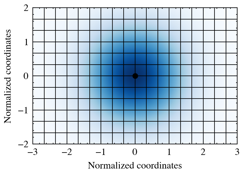
The figure below illustrates a single particle (black), its kernel (blue), and the grid cells receiving contributions.
The central method is deposit_to_grid. The most important arguments include:
fields: the fields to deposit. We can pass a single or a list of fields, either directly, by attribute or by name.averaged: defines which fields represent averaged and cumulative quantities. E.g. when depositing temperatures we want the average in a cell, while mass is a cumulative quantity.gridnums: numbers of grid cells to use in each spatial dimension. If a single number is passed, the code uses this number for every dimension, otherwise, a list of numbers for every axis must be passed.extent: ifboxsizeisNone, this argument must be provided. If provided, deposit particles only within the given extent. Can be used to quickly generate images of subgroups of the cloud.
The following arguments are optional but can be useful in certain situations:
plane_projection: list of axes spanning the projection plane.[0, 1]→ ‘xy’,[2, 1]→ ‘zy’, etc. Useful for projecting 3D particle clouds to 2D and depositing onto a 2D grid.return_weights: whether to return the aggregated particle weights in each cell.integration_method: one of'midpoint','trapezoidal','simpson'. Determines which numerical quadrature to use when integrating kernels over grid cells. Only relevant forisotropicandanisotropic, since integrals ofseparablekernels are analytically evaluated.eta_crit: parameter controlling anti-aliasing.
An example workflow may look like the following example. For more detailed workflows refer to the tutorial sections.
kwargs = {
    fields=[f, self.velocity, 'temperature'],
    averaged=[False, True, True],
    gridnums=[100, 128, 256],
    kernel_name='gaussian',
    return_weights=True,
}

fields_grid, weights_grid = pc.deposit_to_grid(  # shapes: (128, 128, 128, 3), (128, 128, 128)
    **kwargs,
    structure='isotropic',
)

fields_grid, weights_grid = pc.deposit_to_grid(  # shapes: (128, 128, 3), (128, 128)
    **kwargs,
    extent=[boxsize/4, boxsize/2, boxsize/4, boxsize/2]
    structure='anisotropic',
    plane_projection=[0, 1],
)