Gradient fields

In this tutorial we will see how we can chain together the interpolation and deposition modes in smudgy.

• First, we will compute the gradient of a particle field

• Then, we deposit the newly computed gradients to a 2D grid

Interpolating particle gradients and depositing them

First, let’s load all the necessary packages and modules.

import matplotlib.pyplot as plt
import numpy as np
import smudgy as sm

np.random.seed(0)

Show code cell source

Hide code cell source

try:
    plt.style.use('custom')
except:
    pass
%matplotlib inline
%config InlineBackend.figure_format='retina'

Then, we initialize a (random) 2D particle cloud in a periodic box of size 1, and globally set an isotropic cubic kernel and set the number of neighbors to 32. We also assign to each particle an internal energy value \(u\):

boxsize = 1.0
N = 1000
positions = np.random.uniform(0.0, boxsize, size=(N, 2))
weights = np.ones(N)

pc = sm.PointCloud(positions,
                   weights,
                   boxsize=boxsize).\
    global_setup(kernel_name='cubic_spline',
                 structure='isotropic',
                 num_neighbors=32)

# add field to the point cloud
particle_u = np.random.normal(loc=10, scale=1, size=N)
particle_u = np.clip(particle_u, 0.0, None)

pc.add_fields('internal_energy', particle_u)

[smudgy] Initialized 2d PointCloud with 1000 particles in periodic box of size=[1. 1.]
[smudgy] Set structure globally to 'isotropic'
[smudgy] Set kernel globally to 'cubic_spline'
[smudgy] Set number of neighbors globally to 32

Next, we compute smoothing lenghts and densities with the globally set parameters:

pc.compute_smoothing()
pc.compute_density()

[smudgy] Building kd-tree from particle positions
[smudgy] Computing smoothing lengths from 32 neighbors
[smudgy] Computing density using isotropic 'cubic_spline' kernel

Now we can compute (interpolate) the energy gradients at the particle positions. We do so by not passing query_positions, which will default to use pc.positions:

energy_gradient = pc.interpolate_fields(
    fields=['internal_energy'],
    compute_gradients=True) # shape = (N, 1, 2)

[smudgy] Interpolating gradients of fields at query positions using isotropic 'cubic_spline' kernel

We register the newly computed gradient field to the point cloud instance:

pc.add_fields('internal_energy_gradient', energy_gradient[:, 0, :])

Now we can access that gradient field by name to deposit it to a uniform 2D grid of 256 cells on each side:

nx = 256

grid_gradients = pc.deposit_to_grid(
    fields=['internal_energy_gradient'],
    structure='isotropic',
    averaged=True,
    gridnums=nx,
    omp_threads=4
    ) # shape = (nx, nx, 2)

[smudgy] Using c++ backend for isotropic deposition (isotropic_2d)

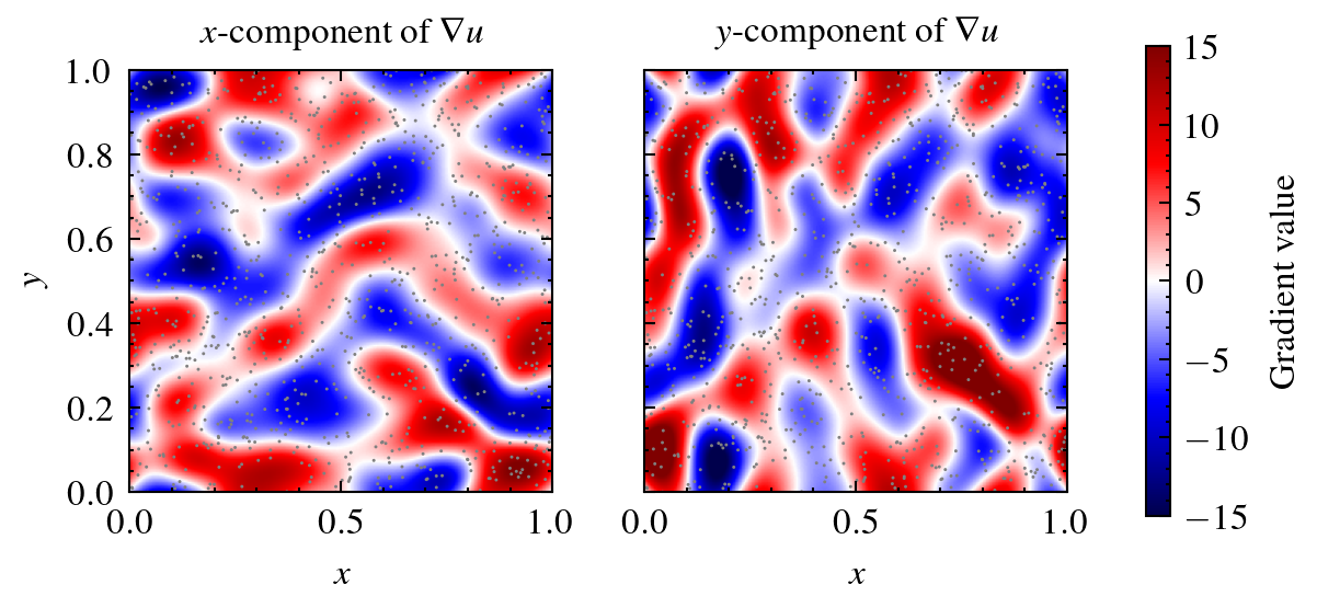
Finally, we visualize the two gradient components side-by-side together with the particles shown in gray:

Show code cell source

Hide code cell source

kwargs = dict(
    extent =[0, boxsize, 0, boxsize],
    vmin = -15,
    vmax = 15,
    cmap = 'seismic'
)

fig, ax = plt.subplots(
    1, 2,
    figsize=(4, 2),
    sharex=True,
    sharey=True,
    constrained_layout=True,
)

im = ax[0].imshow(grid_gradients[..., 0], **kwargs)
ax[1].imshow(grid_gradients[..., 1], **kwargs)

ax[0].scatter(positions[:, 0], positions[:, 1], s=2, alpha=1, color='gray', ec='none')
ax[1].scatter(positions[:, 0], positions[:, 1], s=2, alpha=1, color='gray', ec='none')

for a in ax:
    a.set_xlabel(r'$x$')
ax[0].set_ylabel(r'$y$')

ax[0].set_title(r'$x$-component of $\nabla u$')
ax[1].set_title(r'$y$-component of $\nabla u$')
fig.colorbar(im, ax=ax, shrink=0.8, label=r'Gradient value')

fig.savefig("gradients.png", dpi=300, bbox_inches="tight")
plt.close()

Note

Gradients computed with this method are different compared to gradients of grids:

• Depositing per‑particle gradients preserves the local gradient estimates computed at particle scales and then averages them into cells.

• Computing the gradient of the deposited scalar field (e.g. via finite‑differences) produces a different result because of cell averaging and the finite‑difference operator, i.e.

  \[ \mathrm{deposit} (\nabla f) \neq \nabla(\mathrm{deposit}(f)). \]

Use the first for particle‑scale gradient estimates and the second when you prefer derivatives computed on the (possibly smoothed) grid representation.