Numerical Quadrature
This tutorial introduces numerical quadrature and how it affects depositing particle quantities onto grids in smudgy. We also discuss the different options available.
In the context of smudgy, deposition is the process of mapping continuous particle kernels onto a discrete grid. Mathematically, this involves computing the integral of the kernel function for particle \(p\) over the \(i\)-th cell domain:
Evaluating this integral exactly is often difficult or computationally expensive, especially for complex kernels or anisotropic shapes. Numerical quadrature approximates this integral by evaluating the kernel function at specific points within the cell.
Generally, smudgy focuses on three central aspects regarding its numerical integration schemes: accuracy, conservation of particle mass (or weight) and anti-aliasing.
Accuracy
Currently smudgy supports three numerical integration schemes for approximating the integral of a function \(f(x)\) over a cell of width \(\Delta x\) and center \(x_i\). The formulas represent the methods in 1D:
midpoint: The simplest method. \(f(x)\) is evaluated at the center of each cell. This is the fastest option, but can be less accurate for small smoothing lengths.\[ \int_{x_i - \Delta x/2}^{x_i + \Delta x/2} f(x) dx \approx \Delta x f(x_i)\]trapezoidal: Uses a trapezoidal rule for integration. It evaluates \(f(x)\) at the boundaries and weights them to provide a more accurate estimate of the linear variation.\[ \int_{x_i - \Delta x/2}^{x_i + \Delta x/2} f(x) dx \approx \frac{\Delta x}{2} \left[ f(x_i - \Delta x/2) + f(x_i + \Delta x/2) \right] \]This method reduces error by accounting for the slope between cell boundaries.
simpson: Uses Simpson’s rule, which approximates the integrand with a quadratic polynomial. It is generally the most accurate of the three but requires more function evaluations.\[ \int_{x_i - \Delta x/2}^{x_i + \Delta x/2} f(x) dx \approx \frac{\Delta x}{6} \left[ f(x_i - \Delta x/2) + 4f(x_i) + f(x_i + \Delta x/2) \right] \]By using both the center and the boundaries, it achieves higher-order precision for smooth functions.
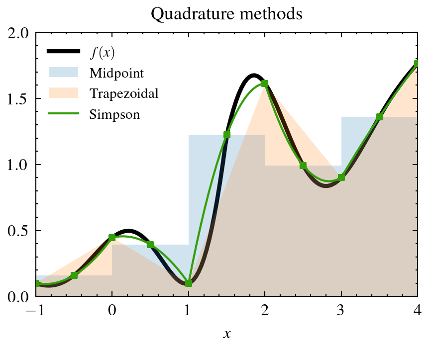
The figure below offers a visual representation of the three methods described above:
Conservation of mass
When integrating kernel functions for deposition purposes with isotropic or anisotropic kernels, the integrals are approximated by one of the above methods. SPH kernels are defined and normalized over a compact support region \(\Omega_s\), i.e.
Any numerical deviation from this normalization implies that the total mass or weight of particles is not globally conserved after depositing to grid, which is unwanted behavior for many physical applications. This constraint is so important, that smudgy tracks the total deposited weight per particle and corrects the total contribution via the following re-weighting scheme:
# for every particle
tracked_weights = 0.0
for cell in Omega_s:
    cell_integral = quadrature(kernel, cell) # approximative
    tracked_weights += cell_integral

correction_factor = 1.0 / tracked_weights
for cell in Omega_s:
    cell_integral *= correction_factor
While this scheme may slightly distort relative integral contributions to cells, it ensures the central constraint of mass conservation exactly!
Anti-aliasing
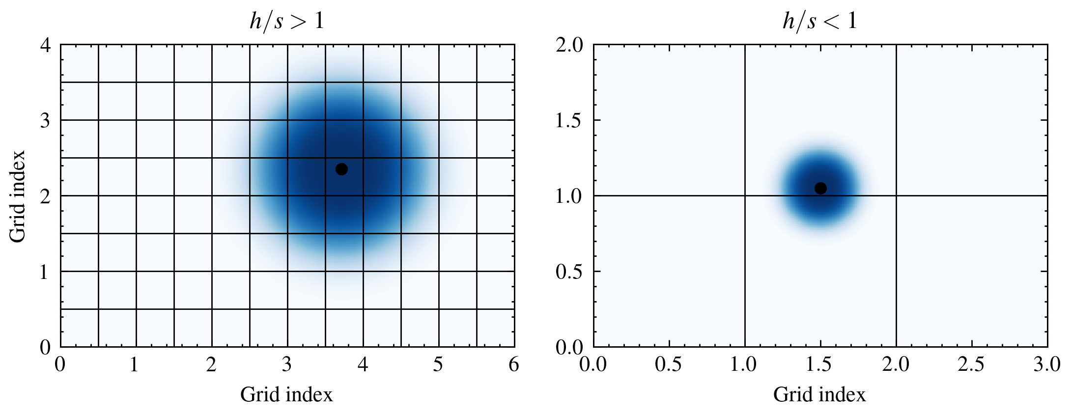
In the context of grid deposition, anti-aliasing refers to the problem of integrating particle kernels whose extent is smaller than the grid cell size, upon which we evaluate the numerical quadrature method. The image below shows two example cases that can occur when depositing. For the left case the ratio of kernel size (~\(h\)) and grid spacing \(s\) is large enough and numerical qudrature can be used. On the right, the kernel affects two cells, while its size is much smaller than \(s\). Integral estimations using the any of the qudrature methods would yield a vanishing integral for both cells.
To combat such cases, the anti-aliasing strategy in smudgy is simple: for every particle the code compares \(\eta = h/s\) to a critical value \(\eta_{\rm crit}\) set by the user (eta_crit=1.0 by default). If \(\eta > \eta_{\rm crit}\), the kernel typically spans over many cells and the integral is estimated via numerical quadrature. If \(\eta < \eta_{\rm crit}\), the code uses pre-computed integral samples and deposits them into the corresponding cells. The threshold where this switch happens can be controlled via the eta_crit argument in deposit_to_grid, while the number of integral samples to use per axis is set by num_kernel_evaluations_per_axis (default 4).
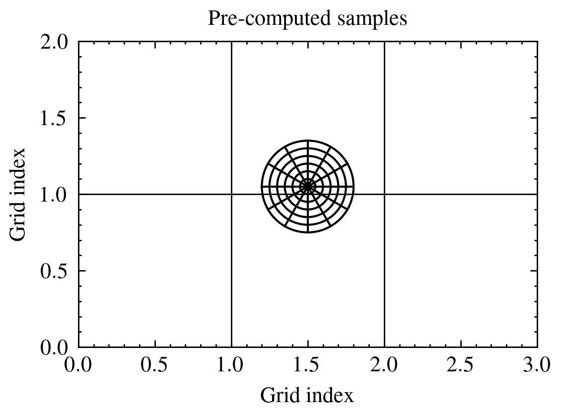
Before deposition, smudgy internally constructs a sample grid depending on the number of num_kernel_evaluations_per_axis. Below we show a visual representation by setting this parameter to 6. The code then precomputes the exact integrals for each sample bin. When samples are used to approximate the integral, the code assigns each precomputed value to the grid cell into which the sample falls. This method is very fast and suitable for most applications. In principle, we can increase the number of evaluations for more accurate quadrature, but we should keep in mind that the cost grows quadratically for 2D and cubically for 3D.