Exploring kernel functions

In this tutorial we will see all kernel functions currently available in smudgy. We will deposit a particle dataset from a cosmological N-body simulation with different kernels and investigate the advantages of certain kernels wrt. dynamic range and power spectrum analysis.

First, let’s load all necessary packages and modules.

import numpy as np
import matplotlib.gridspec as gridspec
import matplotlib.pyplot as plt
import smudgy as sm
from smudgy import get_kernel_shapes_1D
from powerbox import get_power

Show code cell source

Hide code cell source

try:
    plt.style.use('custom')
except:
    pass
%matplotlib inline
%config InlineBackend.figure_format='retina'

As discussed in the Kernels and Structures wiki page, smudgy supports separable, iso- and anisotropic structures. Currently, only tophat, tsc and gaussian kernels can be used for separable structures, while all kernels can be used for the other two.

Let’s define the structures and a dict with kernel names to analyze.

structures = ['separable', 'isotropic', 'anisotropic']

kernel_names = {
    "Tophat": "tophat",
    "TSC": "tsc",
    "Gaussian": "gaussian",

    "Lucy": "lucy",
    "Cubic Spline": "cubic_spline",
    "Quintic Spline": "quintic_spline",

    "Wendland C2": "wendland_c2",
    "Wendland C4": "wendland_c4",
    "Wendland C6": "wendland_c6",
}
batch_1 = {name: kernel_names[name] for name in list(kernel_names.keys())[0:3]}
batch_2 = {name: kernel_names[name] for name in list(kernel_names.keys())[3:6]}
batch_3 = {name: kernel_names[name] for name in list(kernel_names.keys())[6:9]}
batches = [batch_1, batch_2, batch_3]

colors = plt.rcParams['axes.prop_cycle'].by_key()['color'][:len(kernel_names.keys())]

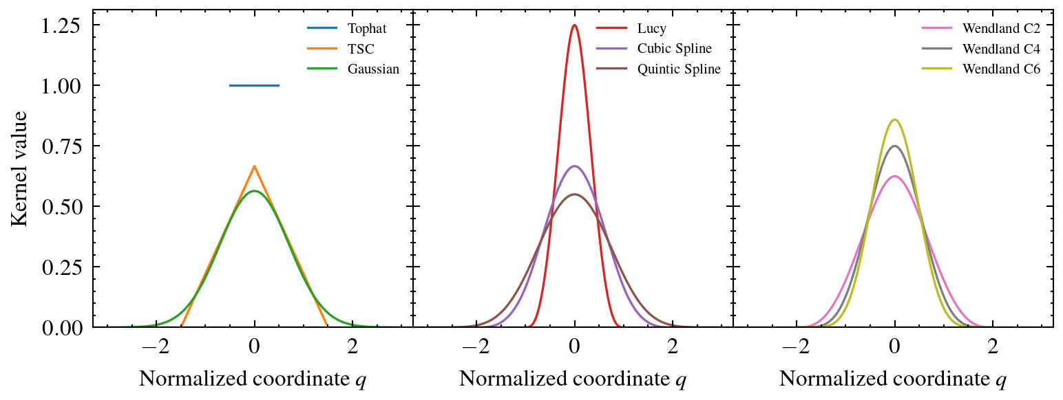
Kernel shape comparison

The following figure shows a comparison of all available 1D kernel functions in smudgy, where the normalized coordinate \(q=|r|/h\).

Show code cell source

Hide code cell source

fig, ax = plt.subplots(1, len(batches), sharex=True, sharey=True, figsize=(6, 2))

c = 0
for i, batch in enumerate(batches):
    for kernel_name, kernel_key in batch.items():
        q, values = get_kernel_shapes_1D(kernel_key)
        ax[i].plot(q, values, label=kernel_name, lw=0.8, color=colors[c])
        c += 1
    ax[i].legend(fontsize=5, loc='upper right')
    ax[i].set_xlabel(r"Normalized coordinate $q$")

ax[0].set(
       ylabel="Kernel value",
       ylim=(0, None)
       )

fig.savefig("kernel_shapes.png", dpi=300, bbox_inches="tight")
plt.close()

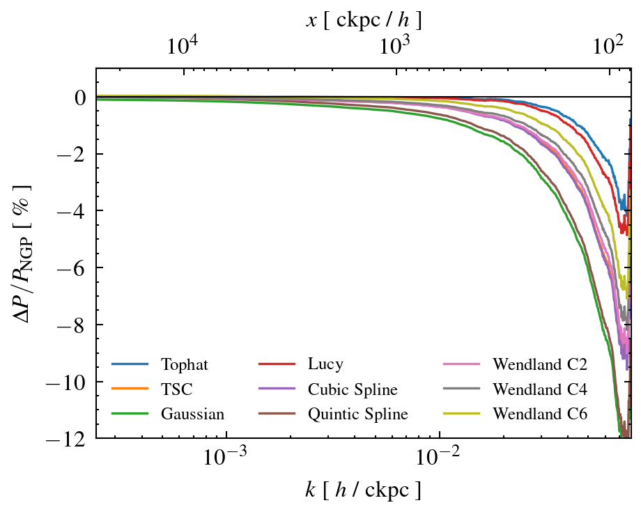
Effect of kernel shape on Power Spectrum

Different kernels are defined over different support domains. Some kernels exhibit sharper and more concentrated shapes, while others are more smoothly extended. Therefore, interpolation and deposition results almost always depend on the chosen kernel. We demonstrate this in the following workflow, where we deposit particles from a cosmological N-body simulation using different kernel functions.

First, we compute a reference grid using Nearest Grid Point assignment (NGP), which is often used in such applications. Then, with NGP as the baseline we compare the results by using higher order kernels and finally show the relative difference on the power spectrum.

We use the TNG50-4-Dark simulation from the publically available TNG runs as well as the illustris_python package to load positions, masses and the boxsize information.

Show code cell source

Hide code cell source

import illustris_python as il

basePath = '/Users/mauro/work/projects/smudgy/data/tng_dark_snapshot_0/'
snapNum = 99
boxsize = 35_000
dm = il.snapshot.loadSubset(basePath, snapNum, "dm")

positions = dm['Coordinates']
masses = np.ones(len(positions)) * 0.0186754872146347 * 1e10 # in Msun/h
positions = np.clip(positions, 0.1, boxsize-0.1)

Then we initialize a PointCloud object, set some parameters to use during later computations and compute the smoothing lengths. For this tutorial we use isotropic structures.

cloud = sm.PointCloud(
    positions=positions,
    weights=masses,
    boxsize=boxsize
    )

gridnums = 512
num_neighbors = 16

kwargs = dict(
    fields=cloud.weights,
    averaged=False,
    gridnums=gridnums,
    eta_crit=10, # due to anti-aliasing for tophat kernel
    omp_threads=10,
)

cloud.global_setup(num_neighbors=num_neighbors, structure='isotropic')
cloud.compute_smoothing()

[smudgy] Initialized 3d PointCloud with 19683000 particles in periodic box of size=[35000 35000 35000]
[smudgy] Set structure globally to 'isotropic'
[smudgy] Set number of neighbors globally to 16
[smudgy] Building kd-tree from particle positions
[smudgy] Computing smoothing lengths from 16 neighbors

Next we compute the reference grid using NGP and perform the depositions by looping over the different kernels.

f_ref = cloud.deposit_to_grid(
    **kwargs,
    kernel_name='ngp',
)[..., 0]

maps = []
for kernel_name, kernel_key in kernel_names.items():

    f = cloud.deposit_to_grid(
        **kwargs,
        kernel_name=kernel_key,
    )[..., 0]
    maps.append(f)

[smudgy] Using c++ backend for ngp deposition (ngp_3d)
[smudgy] Using c++ backend for isotropic deposition (isotropic_3d)
[smudgy] Using c++ backend for isotropic deposition (isotropic_3d)
[smudgy] Using c++ backend for isotropic deposition (isotropic_3d)
[smudgy] Using c++ backend for isotropic deposition (isotropic_3d)
[smudgy] Using c++ backend for isotropic deposition (isotropic_3d)
[smudgy] Using c++ backend for isotropic deposition (isotropic_3d)
[smudgy] Using c++ backend for isotropic deposition (isotropic_3d)
[smudgy] Using c++ backend for isotropic deposition (isotropic_3d)
[smudgy] Using c++ backend for isotropic deposition (isotropic_3d)

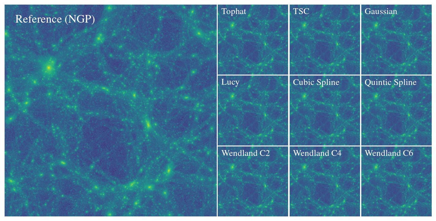
The figure below offers a visual comparison between the different maps.

Show code cell source

Hide code cell source

ref_proj = f_ref.sum(axis=-1)
ref_log = np.log10(ref_proj + 1e-10)
vmin, vmax = ref_log.min(), ref_log.max()

fig = plt.figure(figsize=(6, 3))
gs = gridspec.GridSpec(3, 4, width_ratios=[3, 1, 1, 1], wspace=0.01, hspace=0.01)

# Left Panel: Reference (NGP)
ax_ref = fig.add_subplot(gs[:, 0])
ax_ref.imshow(ref_log.T, origin='lower')
ax_ref.axis('off')
ax_ref.text(0.05, 0.95, "Reference (NGP)", color='white',
            transform=ax_ref.transAxes, va='top', fontsize=9, fontweight='bold')

for i, (name, _) in enumerate(kernel_names.items()):
    row, col = divmod(i, 3)
    ax = fig.add_subplot(gs[row, col+1])

    # Calculate relative difference of the log10 fields
    kernel_proj = maps[i].sum(axis=-1)
    kernel_log = np.log10(kernel_proj + 1e-10)

    # Calculate rel diff: (log_kernel - log_ref) / |log_ref| * 100
    denom = np.abs(ref_log)
    mask = (denom > 1e-12)
    rel_diff = np.zeros_like(kernel_log)
    rel_diff[mask] = (kernel_log[mask] - ref_log[mask]) / denom[mask] * 100

    ax.imshow(kernel_log.T, origin='lower', vmin=vmin, vmax=vmax)
    ax.text(0.05, 0.95, name, color='white', transform=ax.transAxes, va='top', fontsize=7)
    ax.axis('off')

fig.savefig("kernel_projection_comparison.png", dpi=300, bbox_inches="tight")
plt.close()

Next, we use the get_power function from the powerbox package to compute power spectra for the baseline and kernel maps.

pk_ref, k_ref = get_power(f_ref, boxlength=boxsize)

power_spectra = []
for f in maps:
    p, k = get_power(f, boxlength=boxsize)
    power_spectra.append(p)

Show code cell output

Hide code cell output

/opt/anaconda3/envs/my_env/lib/python3.12/site-packages/powerbox/tools.py:261: FutureWarning: In the future, bins will be generated by default up to the smallest length over any dimension, instead of the largest magnitude for the box.Set bins_upto_boxlen to silence this warning.
  bins = _getbins(bins, coord_mags, log_bins, bins_upto_boxlen=bins_upto_boxlen)

Finally we compare the power spectra wrt. the baseline (NGP). For the chosen deposition parameters, we see that different kernels can have a relatively large impact (order percentage) especially on scales \(x \leq 1 \, \mathrm{cMpc}/h\)

Show code cell source

Hide code cell source

def relative_difference(a, b):
    # Avoid division by zero
    mask = (b != 0)
    res = np.zeros_like(a)
    res[mask] = (a[mask] - b[mask]) / b[mask] * 100
    return res

def k2x(k):
    return 2 * np.pi / k

def x2k(x):
    return 2 * np.pi / x

fig, ax = plt.subplots()
for i, (name, _) in enumerate(kernel_names.items()):

    # relatvie difference to reference
    rel_diff = relative_difference(power_spectra[i], pk_ref)

    ax.semilogx(k, rel_diff, label=name, lw=0.8, color=colors[i])

ax_top = ax.secondary_xaxis('top', functions=(k2x, x2k))
ax_top.set_xlabel(r"$x$ [ ckpc / $h$ ]")
ax_top.tick_params(which='both', top=True, labeltop=True)
ax.tick_params(which='both', top=False, labeltop=False)

ax.axhline(0, color='k', linestyle='-', lw=0.5)
ax.legend(fontsize=6, ncols=3, loc='lower left')
ax.set(xlim=(k_ref.min(), k_ref.max()),
       ylim=(-12, 1),
       xlabel=r"$k$ [ $h$ / ckpc ]",
       ylabel=r"$\Delta P / P_{\rm NGP}$ [ \% ]",
       )

fig.savefig("kernel_power_comparison.png", dpi=300, bbox_inches="tight")
plt.close()

Show code cell output

Hide code cell output

/var/folders/g9/6lkt0k991jsbvwhk4pft359m0000gn/T/ipykernel_31506/1144763928.py:12: RuntimeWarning: divide by zero encountered in divide
  return 2 * np.pi / x