Projections

This tutorial showcases how to deposit 3D particle fields onto 2D projection planes.

• We showcase this workflow both for isotropic and anisotropic structures

• We will introduce the math behind the projection engine in smudgy, and how it relates to relevant methods and parameters

import matplotlib.pyplot as plt
import numpy as np
import smudgy as sm

np.random.seed(0)

Show code cell source

Hide code cell source

try:
    plt.style.use('custom')
except:
    pass
%matplotlib inline
%config InlineBackend.figure_format='retina'

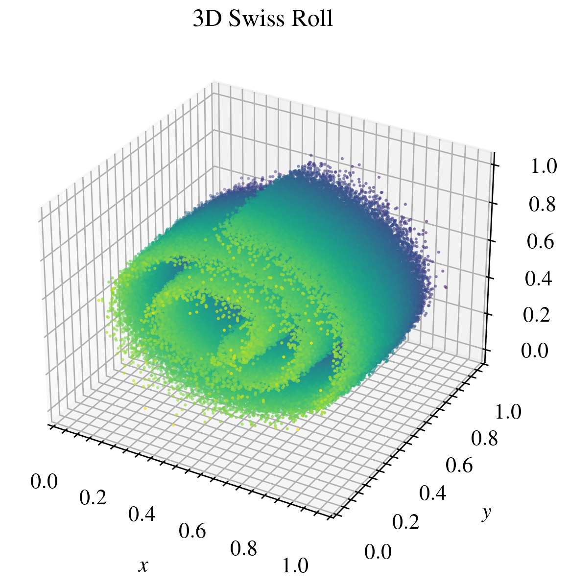
We will use the 3D swiss role dataset with the following parameters:

# Swiss roll parameters
height = 1.0
length = 5 * np.pi
noise  = 0.5

N = 500_000
weights = np.ones(N)

# Generate 3D Swiss roll dataset
t = length * (np.random.rand(N)) + 1.5 * np.pi  # t in [1.5pi, 3pi]
x = t * np.cos(t)
y = height * np.random.rand(N)
z = t * np.sin(t)

# Add noise
x += noise * np.random.randn(N)
y += noise * np.random.randn(N)
z += noise * np.random.randn(N)

# Rescale to [0, 1]
X_swiss = np.vstack((x, y, z)).T
min_X = X_swiss.min(axis=0)
max_X = X_swiss.max(axis=0)
positions = (X_swiss - min_X) / (max_X - min_X + 1e-8)* 0.99

Show code cell source

Hide code cell source

fig = plt.figure(figsize=(4, 3))
ax = fig.add_subplot(projection='3d')

ax.scatter(positions[:, 0],
           positions[:, 1],
           positions[:, 2],
           marker='.',
           s=5,
           edgecolors='none',
           c=-positions[:, 1],
           cmap='viridis',
           )

ax.set_title('3D Swiss Roll', fontsize=9)
ax.set_xlabel(r'$x$')
ax.set_ylabel(r'$y$')
ax.set_zlabel(r'$z$')

plt.tight_layout()
plt.show()

Next, we initialize a point cloud instance in an open box with weights set to ones, a quintic spline kernel and 32 nearest neighbors to use during operations:

pc = sm.PointCloud(positions=positions, weights=weights)\
    .global_setup(kernel_name='quintic_spline', num_neighbors=32)

[smudgy] Initialized 3d PointCloud with 500000 particles without periodicity
[smudgy] Set kernel globally to 'quintic_spline'
[smudgy] Set number of neighbors globally to 32

Next, we compute all the relevant smoothing quantities both for isotropic and anisotropic structures:

pc.compute_smoothing(structure='isotropic')
pc.compute_smoothing(structure='anisotropic')

[smudgy] Building kd-tree from particle positions
[smudgy] Computing smoothing lengths from 32 neighbors
[smudgy] Computing smoothing tensors from 32 neighbors

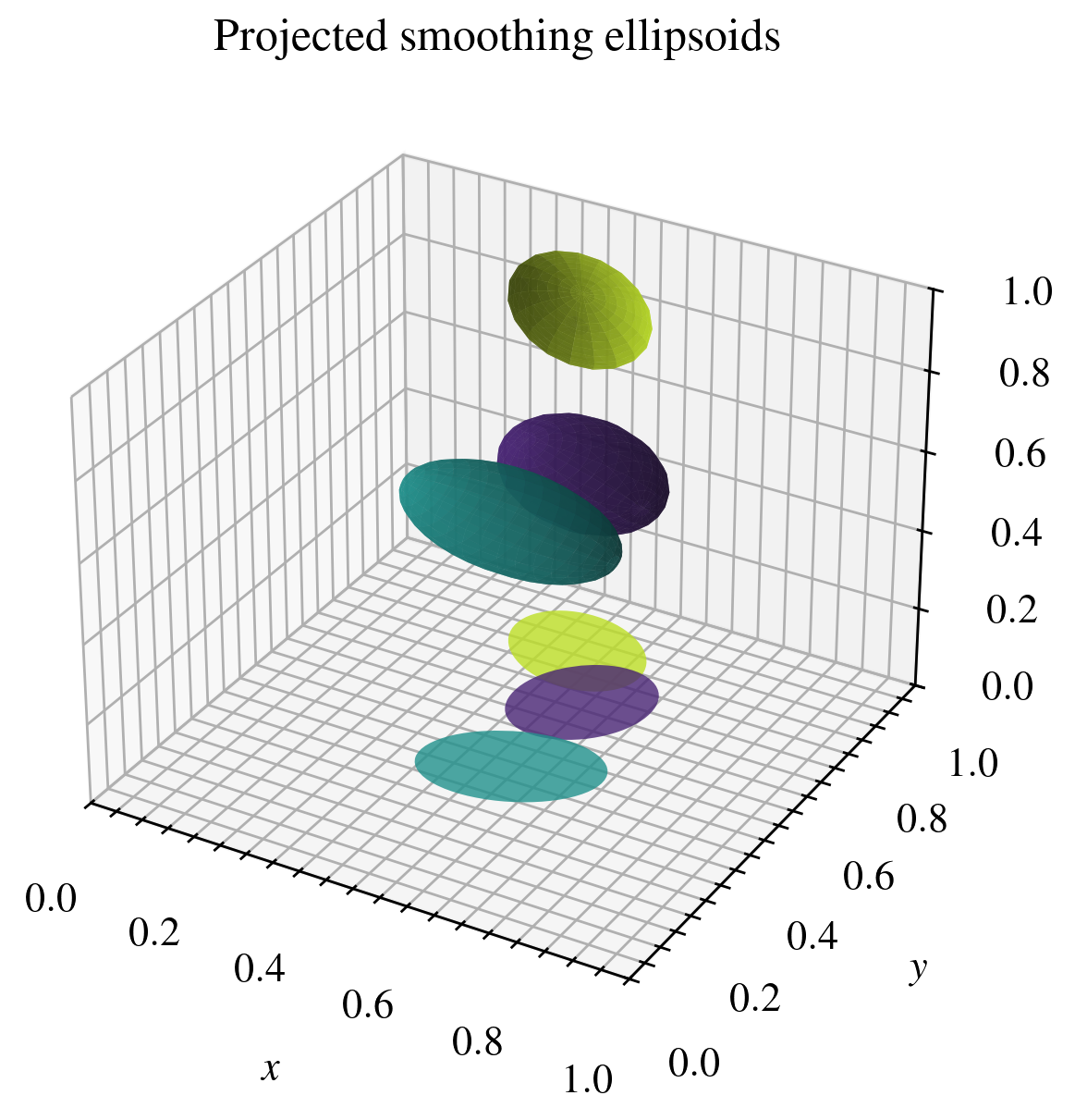
A note on projecting smoothing tensors

Projecting a 3D smoothing tensor \(H \in \mathbb{R}^{3\times 3}\) into a 2D plane proceeds by working with its inverse (a metric form) and restricting it to a chosen subspace spanned by two vectors \(p_1\) and \(p_2\). These basis vectors form the rows of the projection matrix \(P \in \mathbb{R}^{2\times 3}\). The projected smoothing tensor is then computed via a simple matrix multiplication:

\[\begin{split}H_{2D} = \left(P\, H^{-1}\, P^\top\right)^{-1} \qquad \text{where} \qquad P = \begin{bmatrix} p_1^\top \\ p_2^\top \end{bmatrix} \in \mathbb{R}^{2\times 3}. \end{split}\]

The 2D eigenvalues and -vectors are then readily computed from the projected smoothing tensor.

Below we show a visual example of projecting smoothing ellipsoides defined by \(H\) onto the \(x-y\) plane.

Show code cell source

Hide code cell source

from helpers import plot_projection_demo

fig, ax3d = plot_projection_demo(N=3, projection_plane='xy')
plt.tight_layout()
plt.show()

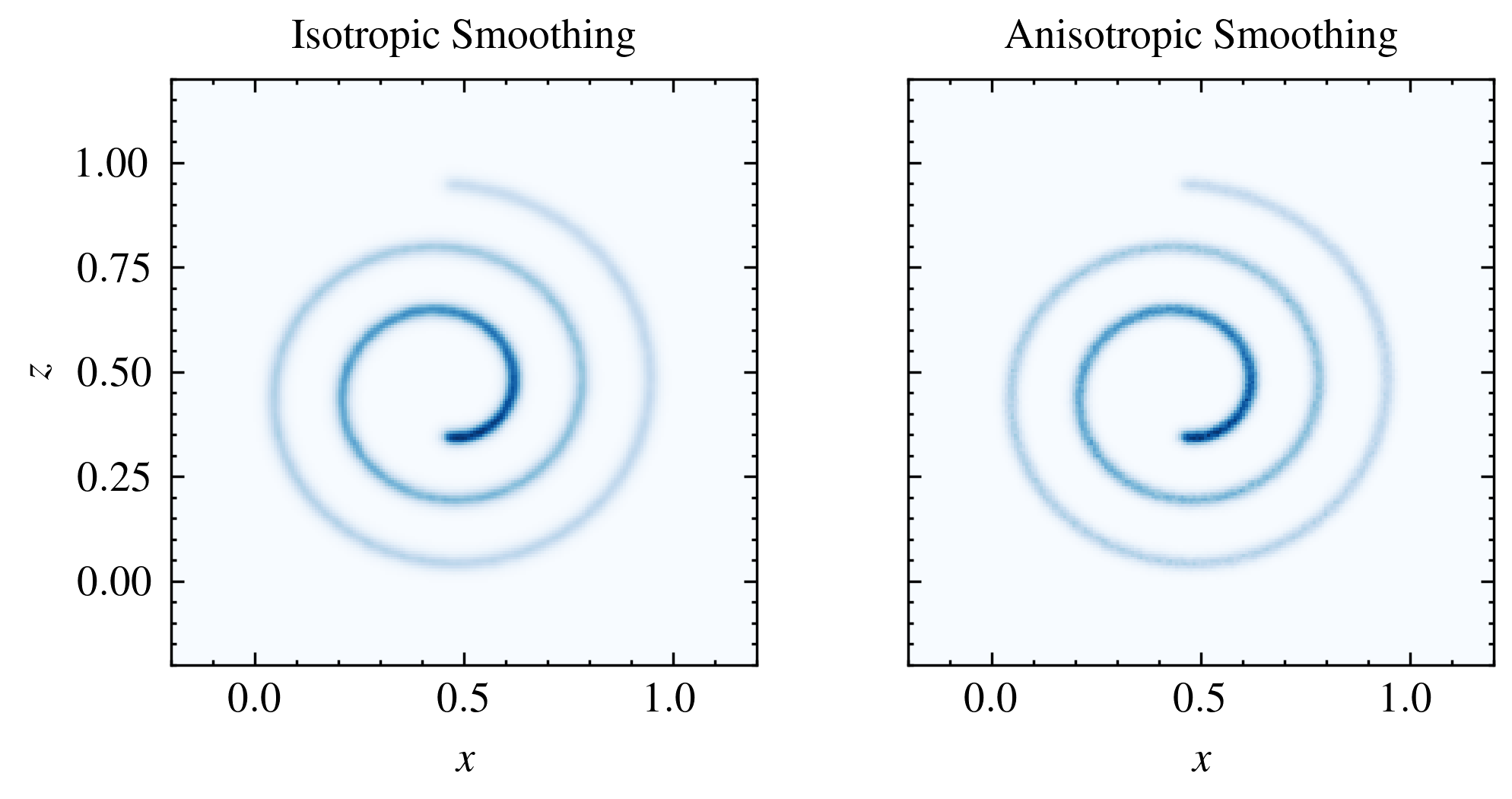
Projected depositions in smudgy

Now we will deposit the particle weight field to a 2D grid by projecting the smoothing lengths and tensors onto the relevant projection planes. Currently, only projection planes spanned by two of the three cartesian axes are possible. Users can simply pass a list or tuple of axis indices as the plane_projection argument. E.g. plane_projection=[0, 1] will project onto the \(x-y\) plane, while plane_projection=[2, 1] will project onto the \(z-y\) plane.

buffer = 0.2
kwargs = dict(
    fields=['weights'],
    averaged=False,
    gridnums=200,
    extent=[[-buffer, height+buffer], [-buffer, height+buffer], [-buffer, height+buffer]],
)

grid_2d_iso = pc.deposit_to_grid(
    **kwargs,
    structure='isotropic',
    plane_projection=[0, 2],
)

grid_2d_aniso = pc.deposit_to_grid(
    **kwargs,
    structure='anisotropic',
    plane_projection=[0, 2],
)

[smudgy] Using c++ backend for isotropic deposition (isotropic_2d)
[smudgy] Using c++ backend for anisotropic deposition (anisotropic_2d)

Show code cell source

Hide code cell source

fig, ax = plt.subplots(1, 2, figsize=(5, 2), sharex=True, sharey=True)

kwargs = dict(
    extent = [-buffer, height+buffer, -buffer, height+buffer],
    cmap = 'Blues'
)

ax[0].imshow(np.rot90(grid_2d_iso),
             **kwargs
             )

ax[1].imshow(np.rot90(grid_2d_aniso),
             **kwargs
             )
ax[0].set_xlabel(r'$x$')
ax[0].set_ylabel(r'$z$')
ax[1].set_xlabel(r'$x$')

ax[0].set_title('Isotropic Smoothing')
ax[1].set_title('Anisotropic Smoothing')

fig.savefig("projection_comparison.png", dpi=500, bbox_inches="tight")