Quick walkthrough

This tutorial walks through the central methods and arguments to build workflows for depositing particle fields onto structured grids.

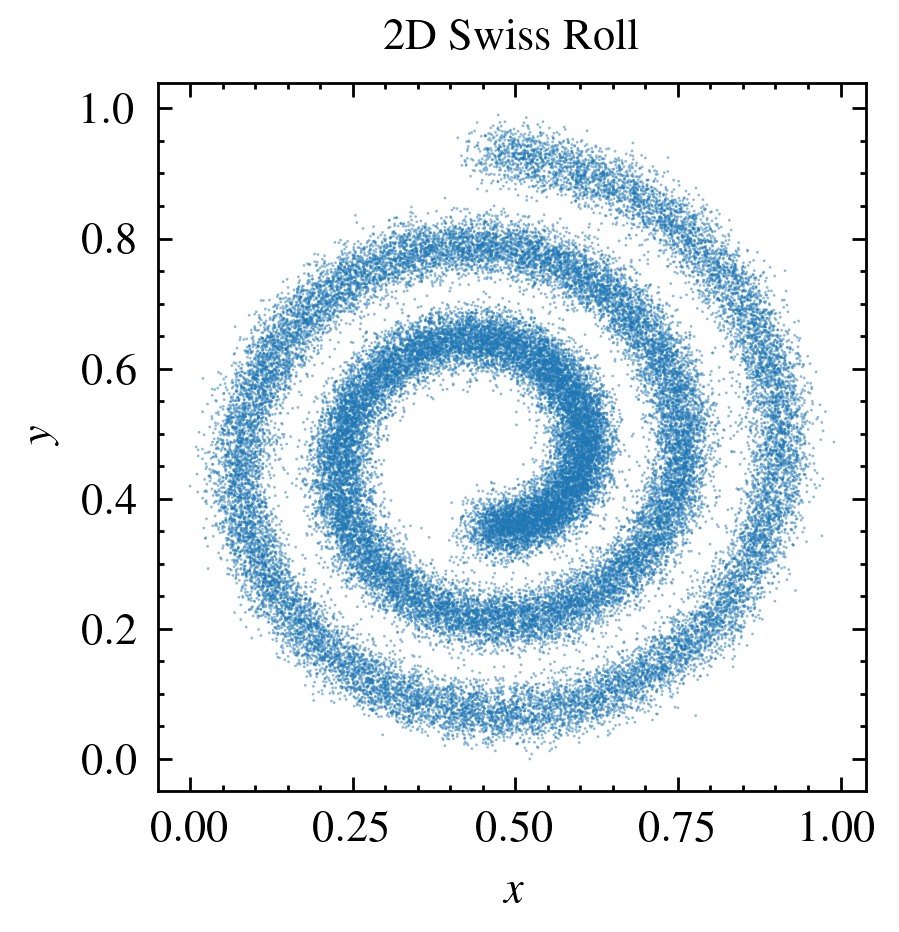
• We will see how to deposit weights of particles drawn from the swiss role dataset onto a uniform 2D grid.

• We will use both isotropic and anisotropic structures for direct comparison.

import matplotlib.pyplot as plt
import numpy as np
import smudgy as sm

np.random.seed(0)

Show code cell source

Hide code cell source

try:
    plt.style.use('custom')
except:
    pass
%matplotlib inline
%config InlineBackend.figure_format='retina'

Depositing a scalar field onto a grid

We will use particles drawn from the swiss role dataset in an open box (i.e. no boxsize parameter is necessary) and weights set to ones:

# Swiss roll parameters
height = 1.0
length = 5 * np.pi
noise  = 1.0

N = 50_000
weights = np.ones(N)

# Generate 2D Swiss roll dataset
t = length * (np.random.rand(N)) + 1.5 * np.pi  # t in [1.5pi, 3pi]
x = t * np.cos(t)
y = t * np.sin(t)

# Add noise
x += noise * np.random.randn(N)
y += noise * np.random.randn(N)

# Rescale to [0, 1]
X_swiss = np.vstack((x, y)).T
min_X = X_swiss.min(axis=0)
max_X = X_swiss.max(axis=0)
positions = (X_swiss - min_X) / (max_X - min_X + 1e-8)* 0.99

Let’s inspect the particle distribution via a simple scatter plot:

Show code cell source

Hide code cell source

fig, ax = plt.subplots()
ax.scatter(positions[:, 0], positions[:, 1], edgecolors='none', s=1, alpha=0.5)
ax.set(xlabel=r'$x$', ylabel=r'$y$', aspect='equal')
ax.set_title('2D Swiss Roll')
plt.show()

Then, we initialize a PointCloud instance and globally set the kernel to a cubic spline and the number of neighbors to use in computations to 32. The structure we do not fix for now as we want to use methods both with isotropic and anisotropic structures.

pc = sm.PointCloud(positions=positions,
                   weights=weights).\
    global_setup(kernel_name='cubic_spline',
                    num_neighbors=32)

[smudgy] Initialized 2d PointCloud with 50000 particles without periodicity
[smudgy] Set kernel globally to 'cubic_spline'
[smudgy] Set number of neighbors globally to 32

Next we compute the smoothing lengths and tensors, by passing the isotropic and anisotropic structure argument to the compute_smoothing method.

pc.compute_smoothing(structure='isotropic')
pc.compute_smoothing(structure='anisotropic')

[smudgy] Building kd-tree from particle positions
[smudgy] Computing smoothing lengths from 32 neighbors
[smudgy] Computing smoothing tensors from 32 neighbors

Since all smoothing information is stored in the pc.smoothing attribute, we can check individual fields:

print('Shape of smoothing lengths:', pc.smoothing.smoLens.shape)
print('Shape of smoothing tensors:', pc.smoothing.smoTens.shape)
print('Shape of smoothing tensor eigenvalues:', pc.smoothing.smoTens_eigvals.shape)
print('Shape of smoothing tensor eigenvectors:', pc.smoothing.smoTens_eigvecs.shape)

Shape of smoothing lengths: (50000,)
Shape of smoothing tensors: (50000, 2, 2)
Shape of smoothing tensor eigenvalues: (50000, 2)
Shape of smoothing tensor eigenvectors: (50000, 2, 2)

Next, let’s assign each particle a field value representing the “energy” \(u\). Here we simply use random numbers and make sure that they are all \(\geq 0\)

particle_u = np.random.normal(loc=1, scale=0.1, size=N)
particle_u = np.clip(particle_u, 0.0, None)

# add them to the point cloud as a field
pc.add_fields('internal_energy', particle_u)

Next, let’s deposit \(u\) onto a uniform 2D grid with 256 cells on each side. We perform this deposition once using isotropic and once anisotropic kernel structures. Note that, since energy is an additive quantitiy (just like e.g. mass), we set averaged=False. Since the point cloud lives in an open, non-periodic box (no boxsize parameter was given during initialization), we need to pass the extent over which the deposition grid should cover:

nx = 256
extent = [[0, height], [0, height]]

grid_isotropic = pc.deposit_to_grid(
    fields=['internal_energy'],
    structure='isotropic',
    averaged=False,
    extent=extent,
    gridnums=nx,
    omp_threads=4
    )

grid_anisotropic = pc.deposit_to_grid(
    fields=['internal_energy'],
    structure='anisotropic',
    averaged=False,
    extent=extent,
    gridnums=nx,
    omp_threads=4
    )

[smudgy] Using c++ backend for isotropic deposition (isotropic_2d)
[smudgy] Using c++ backend for anisotropic deposition (anisotropic_2d)

Let’s visualize the deposited values for both structures as well as the relative difference between the two results. For better visualization, we transform the fields to log-space and compute the relative difference based on the transformed fields:

Show code cell source

Hide code cell source

def relative_difference(a, b):
    return (a - b) / (b + 1e-8)

def transform_image(grid):
    # add a small value to avoid log(0)
    eps = 1e-2
    return np.log10(eps + np.rot90(grid))

grid_isotropic = transform_image(grid_isotropic)
grid_anisotropic = transform_image(grid_anisotropic)


fig, ax = plt.subplots(
    1, 3,
    figsize=(4, 2),
    sharex=True,
    sharey=True,
    constrained_layout=True,
    dpi=300
    )
extent =[0, height, 0, height]

ax[0].imshow(grid_isotropic,
             cmap='Blues',
             extent=extent)
ax[1].imshow(grid_anisotropic,
             cmap='Blues',
             extent=extent)
im = ax[2].imshow(relative_difference(grid_isotropic, grid_anisotropic),
             vmin=-1, vmax=1, cmap='seismic',
             extent=extent)

ax[0].set_title('Isotropic')
ax[1].set_title('Anisotropic')
ax[2].set_title('Relative Difference')

for a in ax:
    a.set_xlabel(r'$x$')
ax[0].set_ylabel(r'$y$')

fig.colorbar(im, ax=ax[2], shrink=0.45)
fig.savefig("comparison.png", dpi=300, bbox_inches="tight")
plt.close()

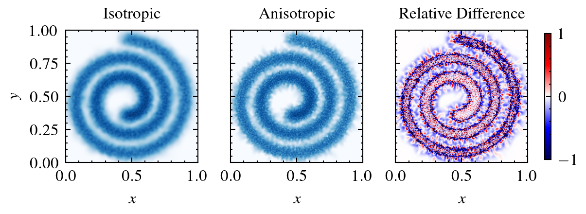
As apparent from the comparison, the anisotropic mode yields much sharper borders around the main spiral. Arguably, the isotropic mode gives better results outside as kernels extend over larger areas and thus yield a smoother representation of the continuous field.