Structure comparison¶

In this tutorial we will investigate the result of different structures in the context of grid deositions. In particular, we use a toy dataset to showcase adaptive and non-adaptive deposition methods supported by clear visualizations of kernel shapes.

In the context of interpolation and/or deposition in smudgy, the concept of adaptivity refers to the choice of whether smoothing lengths should dynamically adapt to the local density environment, or whether they should be treated as fixed numbers.

In smudgy, the latter behaviour can be triggered in the deposit_to_grid function by passing adaptive=False (True by default). In this case, no smoothing is required as the kernel extents are fixed by the grid spacing defined by boxsize or extent and the provided gridnums. This option is particularly useful, if we wish to use non-adaptive deposition algorithms like the widely adapted Cloud-in-Cell (CIC) or Triangular Shaped Cloud (TSC).

The following steps will walk through both options, highlight differences and offer a visual comparison between the two.

First, we import the necessary packages and modules.

import matplotlib.pyplot as plt
import numpy as np
import smudgy as sm

np.random.seed(0)

Next, we initialize the random toy dataset and preset the number of neighbors and grid number parameters. Then we initialize a PointCloud object. For this tutorial we omit periodic boundary conditions. Note that the underlying kernel of the CIC method is the tophat.

# Define parameters for the point cloud
N = 10
boxsize = 1.0
num_neighbors = 3

# Generate random positions and masses for the point cloud
positions = np.random.uniform(0.1 * boxsize, 0.9 *boxsize, (N, 2))

# init smudgy object
cloud = sm.PointCloud(
    positions=positions,
    boxsize=boxsize,
    verbose=False
    ).global_setup(num_neighbors=num_neighbors)

# store fixed kwargs for later use
kwargs = dict(
    fields=cloud.weights,
    averaged=False,
    extent=[[0, boxsize], [0, boxsize]],
    return_weights=True,
    eta_crit=10,
    num_kernel_evaluations_per_axis=32
)

Note that only kernels that have a 1D separable version support the separable, isotropic and anisotropic structures. Currently, these include tophat, tsc and gaussian kernels. The remaining kernels can only be used for isotropic and anisotropic structures.

Regarding adaptivity, the only structures compatible with adaptive=False are

separable: In this case the kernel supports are fixed to the grid spacings for each axis
isotropic: In this case the kernel support is the average of the grid spacings in each dimension

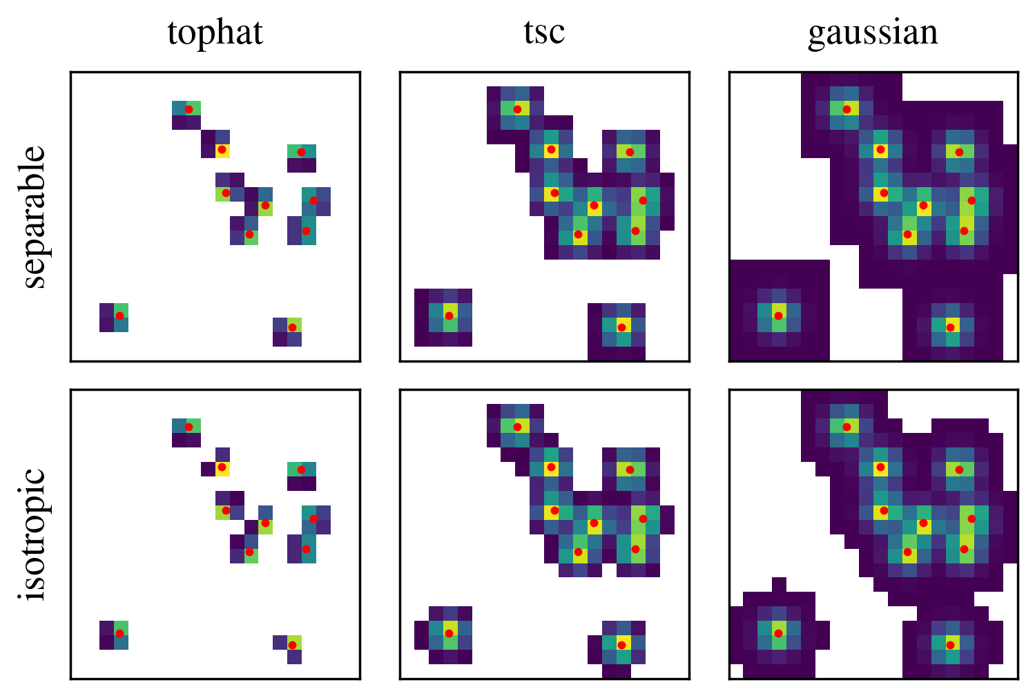
1. Non-adaptive methods¶

Non-adaptive methods such as Cloud-in-Cell or TSC use a fixed kernel size relative to the grid spacing. We can enable such behaviour by setting the adaptive=False in the deposit_to_grid method. This mode is only compatible with separable and isotropic structures.

For better visualization results, we set the background from 0 to NaN.

ADAPTIVE = False

gridnums = 20
structures = ['separable', 'isotropic']
kernel_names = ['tophat', 'tsc', 'gaussian']

maps = []
for i, structure in enumerate(structures):
    for j, kernel_name in enumerate(kernel_names):

        _, weight = cloud.deposit_to_grid(
            **kwargs,
            
            gridnums=gridnums,
            kernel_name=kernel_name,
            structure=structure,
            adaptive=ADAPTIVE,
        )

        F = weight
        F = np.where(F == 0, np.nan, F)
        maps.append(F)

Caution

While it is possible, it is generally not recommended to use isotropic kernels with adaptive=False since severe anti-aliasing effects can occur. Set eta_crit and num_kernel_evaluations_per_axis to higher numbers (e.g. 10 and 32) in this case.

2. Adaptive methods¶

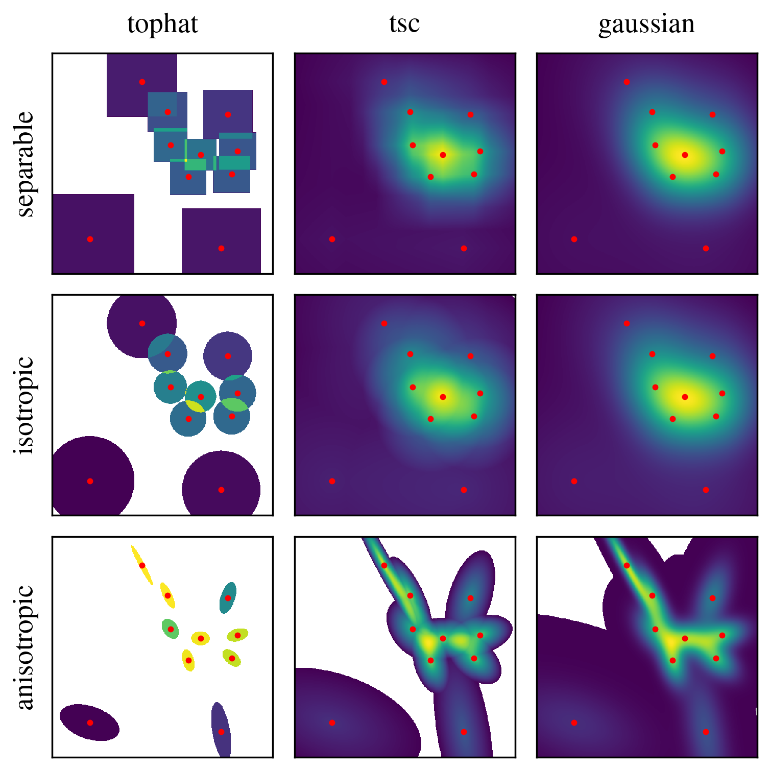
The adaptive option exists for all structures and kernels, and is the default behaviour in smudgy. The comparison plot below showcases the underlying kernel structures by visualizing the deposited weight in each cell. Note that here we use the default values for eta_crit and num_kernel_evaluations_per_axis.

ADAPTIVE = True

gridnums = 512
structures = ['separable', 'isotropic', 'anisotropic']
kernel_names = ['tophat', 'tsc', 'gaussian']

maps = []
for structure in structures:
    
    cloud.compute_smoothing(structure=structure)
    
    for kernel_name in kernel_names:
        
        _, weight = cloud.deposit_to_grid(
            **kwargs,

            gridnums=gridnums,
            kernel_name=kernel_name,
            structure=structure,
            adaptive=ADAPTIVE,
        )

        F = weight
        F = np.where(F == 0, np.nan, F)
        maps.append(F)

fig, ax = plt.subplots(
    len(structures),
    len(kernel_names), 
    figsize=(3, 3),
    sharex=True, 
    sharey=True,
    layout='constrained'
    )

c = 0
for i, structure in enumerate(structures):
    for j, kernel_name in enumerate(kernel_names):
        F = maps[c]
        ax[i, j].pcolormesh(F)
        ax[i, j].scatter(positions[:, 1] * gridnums,
                         positions[:, 0] * gridnums,
                         c='r', s=2)
        ax[i, j].set_aspect('equal')
        ax[i, j].set(xticks=[], yticks=[])
        ax[0, j].set_title(f'{kernel_name}')
        c += 1

    ax[i, 0].set_ylabel(f'{structure}')

fig.savefig("adaptive.png", dpi=500, bbox_inches="tight")
plt.close()